

slsML: Towards elastic ML infrastructure on AWS Lambda


This article was originally written by Alex Glikson on Medium. Reposted with permission.
The seamless elasticity of ‘serverless’ Function-as-a-Service (FaaS) platforms such as AWS Lambda made them an attractive target for a growing variety of applications, such as web backends, ETL, CI/CD, IoT and many others. In the scientific community, AWS Lambda has been used as a general-purpose parallel computation platform, with projects like PyWren. Furthermore, with the growing demand for efficient cloud hosting of Machine Learning (ML) workloads, there are multiple serverless implementations of model inference (e.g., [1], [2], [3], [4]).
As part of our experiments with elastic infrastructure for ML here at Carnegie Mellon, we decided to explore the question whether rapidly elastic serverless platforms (such as AWS Lambda) can be used efficiently for additional kinds of ML workloads, such as distributed training of Deep Learning models.
TL; DR: Overall, we feel that this is still an open research question.
Problem statement
Deep Learning has been successfully applied to many important ML problems, such as image classification. For example, ResNet-50 is a Convolutional Neural Network (CNN) implementation that can be trained on ImageNetdataset (comprising millions of labeled examples) to classify images in 1000 categories (animals, plants, vehicles, etc), with high accuracy. Model training often requires thousands of processing hours, typically performed on a cluster of high-end GPU-accelerated machines (model operations can be efficiently parallelized on hundreds or even thousands of cores present on modern GPUs). In such deployments, GPUs perform the actual training logic (calculation of gradients and weights), while CPUs are performing I/O — both loading the training data (training inputs) and exchanging updated weights between workers nodes.
However, sometimes having a fixed-size long-running cluster is not ideal. For example, if we don’t know in advance how many workers are we going to need, or the desired number of workers is likely to change over time (e.g., adaptively). Hence, we decided to design a seamlessly elastic infrastructure for such workloads, leveraging AWS Lambda, S3, and SNS. Although we knew that we can’t use GPUs with AWS Lambda, we thought that the experiment may still result in relevant insights (briefly summarized in this article).
Adjusting ResNet50 training to run on AWS Lambda
When considering options to run training algorithms in parallel on multiple nodes, there are two main approaches:
- Data-parallel — different nodes train the entire model using different portions of the data (and then the results are aggregated)
- Model-parallel — different nodes train different portions of the model (using same or different data)
Furthermore, the training workflow itself essentially comprises two phases:
- Calculate gradients (based on the previous model and current labeled input)
- Update model weights
In our architecture, we perform the gradients calculation (phase 1) using a data-parallel approach, and the weights updates (phase 2) using model-parallel approach. To facilitate the distributed training across many workers/reducers and iterations, all the model artifacts are stored in a shared storage (S3), and the control flow is implemented using API Gateway (also backed by Lambda), SNS notifications and DynamoDB (for ‘bookkeeping’).
The following figures summarize the Data Flow and the Control Flow in the architecture we implemented.
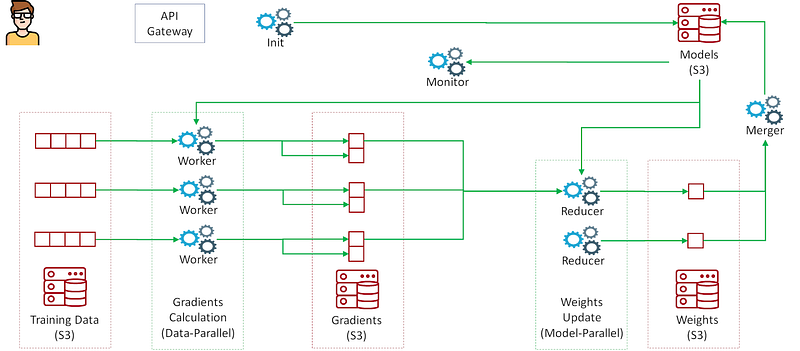
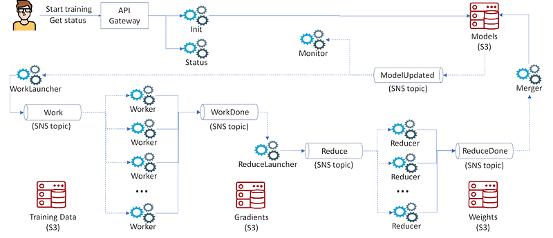
Here is how it works, in a nutshell.
- The workflow is triggered by a (new version of the) model file uploaded to S3, generating an SNS message (ModelUpdated topic) which in turns triggers the WorkLauncher function.
- WorkLauncher is triggering a set of Worker functions by generating an SNS message for each of them, published to the Work topic (Lambda is configured to consume one message per function invocation).
- Each worker is reading the model and the training data from S3, computes and writes gradients back to S3, partitioned per reducer (so that each reducer can then easily access the relevant portion of the gradients). Depending on the number of images in the training set, this can take between few seconds up to several minutes (notice that Lambda is limited to 15 minutes, recently increased from 5 minutes). On completion, each worker notifies ReduceLauncher via SNS topic WorkDone.
- ReduceLauncher keeps track of finishing workers by maintaining a counter in DynamoDB, and triggers reducers by sending the desired number of SNS messages to the Reduce topic once workers are done.
- Reducers read the model and the respective parts of the gradients from S3, compute new weights, write them back to S3, and report completion via ReduceDone topic.
- Triggered via SNS, Merger reads the updated weights and uploads the new model, which triggers WorkLauncher again. Depending on the desired number of iterations (maintained in DynamoDB), WorkLauncher either launches more Workers (step 2), or exits.
Notice that our approach is conceptually similar to map-reduce, but unlike the general case (e.g., implemented by PyWren) we are able to parallelize the aggregation (‘reduce’) phase too, without hitting Lambda runtime limits (i.e., each reducer applies gradients to a dedicated portion of model weights).
The following sections provide more details on the challenges we faced while implementing, debugging and optimizing this architecture.
Working around Lambda runtime limits
Package size
The first challenge was to even get started with running our TensorFlow-based training implementation on Lambda. Standard installation of TensorFlow 1.8 consumes about 400MB of disk space (and growing release-to-release), which is way above Lambda’s current limit (50MB compressed, 250MB uncompressed). So, we had to recompile TensorFlow from source, strip binaries, remove unused packages/modules, as well as to apply ‘minification’ to the native Python code (covering this topic alone would require a separate blog post, as there is no working out-of-the-box solution).
Disk space
Workers, reducers and the merger need to operate on model artifacts persisted in S3. A naive approach might be to use a local filesystem (e.g., /tmp) of individual containers as a buffer. However, on Lambda the disk space in /tmp is limited to 512MB. Hence, somewhat counter-intuitively, it is better to operate with model artifacts directly in memory, where we can allocate up to 3GB of space. Furthermore, since the resource allocation of CPU and RAM on Lambda is proportional (at the moment), and given that our workload is CPU-bound (meaning that the most cost-efficient approach is to allocate the largest possible configuration) — we are essentially getting the largest possible memory allocation almost for free.
Memory
Although memory on Lambda is less limited than disk space, it is still limited to 3GB (at the moment). When a reducer needs to aggregate too many gradients, it will eventually hit this limit. In order to overcome this, we can increase the number of reducers. This way each reducer needs to process a smaller portion of the model. This also slightly decreases reducers’ completion time, given that they operate in parallel (although the runtime of reducers is relatively short, so the benefit is limited).
S3 as distributed shared memory (DSM)
As mentioned above, we use S3 to keep all the model artifacts, throughout the pipelines. This produces a significant traffic to and from S3. For example, with a model size of 180MB, a training set of 1 million images, and each worker running for up to 5 minutes, the pipeline would write and read roughly 1TB of data to/from S3 per epoch (1 pass over training data). Notice that the traffic associated with the actual training data would be orders of magnitude lower. Moreover, if for some reason (e.g., due to mini-batch size limitations) we need to synchronize weights more often — S3 traffic would grow linearly. Besides the direct cost, there are also performance implications of such a solution. For example, it turned out that S3 can sometimes have very large latencies, which caused the so-called ‘stragglers problem’, where the entire pipeline is blocked because of a single S3 access being delayed (more details on this later).
Observability of complex serverless workflows
Once we finished implementing all the pieces of the architecture, there was this awkward moment when we didn’t really know what to do next. So, we put the initial model weights on S3, and we hope that eventually a new model file, with a more accurate model, appears at a designated location. But what if it doesn’t? How do we know if the workflow is actually working correctly? How do we know when something goes wrong? How do we debug it? And on the performance side, how do we know which parts of the workflow are the bottlenecks? How do we optimize? While AWS provides access to basic metrics and logs, it was practically impossible to figure out what is going on. Inevitably, we learned that one of the tough challenges with elastic, event-driven workloads — is observability. So, after searching for available options, we found Epsagon — a really cool serverless tracing and monitoring tool, which aims to do exactly what we needed.
Epsagon
In a nutshell, Epsagon collects tracing data from Lambda functions as well as their CloudWatch logs. Consequently, Epsagon is able to detect runtime properties of individual function invocations (such as resource consumption, errors, timeouts, etc), but more importantly — it instruments and monitors use of common APIs, such as S3 and SNS, and is able to aggregate sequences of related events into ‘transactions’. For example, in our case, an event of uploading a new model file to S3 generates an entire Lambda-based workflow (as outlined above), performing a training iteration involving workers, reducers, launchers, etc, while the various Lambda functions components communicate between them via SNS. Almost magically, Epsagon is able to keep track of this communication and to figure out that all those events are related. Here is an example, with 8 workers, 3 reducers, and model size of 180MB (typical for ResNet-50):

We can see on the diagram the different interactions, their order, how many operations of each kind occurred, as well as their duration. Moreover, we can click on the individual resources, drill down into a specific event (e.g., SNS message JSON, S3 object properties, API call duration, etc), see CloudWatch logs (if this is a Lambda function), and many more.
Epsagon offers lots of other great features too. For example, if there was an error during a function invocation, it will be shown in red in the transaction diagram. Epsagon is also able to send Email alerts for Lambda timeouts, functions killed because they ran out of memory, as well as any Python exceptions. This is especially useful if an application has timer-based workflows (e.g., pre-warming), and you are not monitoring it 24/7.
Epsagon also helps to monitor and predict AWS cost for each function. In our case, the more important cost factor was the human effort — dealing with application complexity, especially during debugging and optimization phases.
Mitigating stragglers
One of the unpleasant surprises that we discovered while debugging the pipeline was the so-called ‘tail latency’ effect, or ‘the straggler problem’. For example, if we have 128 workers, each reducer will need to read 128 files from S3. Files are quite small and S3 is typically very fast — which means that it takes an order of milliseconds to read each file. But this also means that even if we read all the 128 in parallel, and only one of the S3 requests get delayed — the reducer will be waiting. In our experiments, such delays sometimes exceeded 60 seconds — several orders of magnitude longer than normal! Similarly, when, for example, the Merger had to wait for all the reducers to finish — even if only one of them got delayed, so was the entire pipeline. So, we were practically unable to perform any performance tests, because with large concurrency — literally, every run of the pipeline contained at least one such ‘straggler’.
Luckily, given the nature of our application, we don’t really mind losing some small parts of the computation. After all, every weight update produced by every worker/reducer is typically very small. So, we ended up implementing a relaxed synchronization mechanism where we wait only until a certain portion of parallel computations is done (e.g., 90%), essentially replacing a barrier semantics with a counting semaphore. This enabled us to stabilize the pipeline for larger numbers of workers and reducers, with little cost.
Summary of experiments
In order to test the scalability of our solution, and also to explore the tradeoff between cost and elasticity, we ran a series of experiments, with different numbers of workers. For each of them, we calculated the time and the cost it would take to perform one epoch of training (roughly 1 million labeled images), assuming mini-batch size of 8K (found to be empirically feasible) and 32K (hypothetical). Moreover, we compared this to a hypothetical setup in which we have a fixed cluster, and we need to change the size of the cluster (and hence reprovision certain number of VMs) either every 5 minutes or every hour (reflecting different levels of elasticity).

Here are few initial insights (a more detailed analysis is beyond the scope of this article).
Scaling
How well does our solution scale in terms of the number of concurrent workers? Let’s compare it to an ideal solution. In an ideal case, the time to perform a fixed amount of computation (one epoch) will reduce following a 1/x curve, and the cost will be fixed regardless of concurrency.
- Time: We can see on the graph that the time (dotted line) indeed decreases and looks like
1/x, although at around 32 workers it slows down, and stops decreasing at about 256 workers. Looking under the covers, there are two main reasons for such behavior. First, the overhead of maintaining the distributed pipeline and exchanging intermediate results between iterations increases with the number of workers. Second, in order to ensure training convergence, workers need to exchange weight updates in bulks of up to the size of the pre-defined mini-batch (8K or 32K in our case). Therefore, as the concurrency increases, the amount of work each worker can do in an iteration decreases. Hence, we need relatively more iterations, and the per-iteration overhead becomes more significant. - Cost: Looking at the cost (blue and green lines), it indeed remains flat up to a certain point (32 workers for the blue line, 128 for the green one), and then begins to climb. Apparently, there are two main reasons for this. First, due to mini-batch size limit (explained above), the overhead of running the pipeline is higher — which also increases the cost of the corresponding Lambda functions (spending more time waiting). But, interestingly, the main reason for the extra cost is actually the cost of S3 calls, which becomes very significant as the number of workers/reducers increases (notice that the traffic within a region is free, and the only cost is for API calls).
Comparison to a VM-based solution
We compared our Lambda-based implementation to a hypothetical solution based on traditional VM-based distributed training architecture (such as using TensorFlow with a parameter server). We assume that in order to address the need to reconfigure the cluster, we would just re-deploy it, paying the overhead of VMs provisioning and configuration time (typically few minutes). In order to compare the cost, we assume that the overhead of interaction with the parameter server is negligible compared to the provisioning overhead. As shown on the graph, when we need to reconfigure the cluster every 5 minutes, the cost is comparable to our Lambda-based solution (up to the point where it begins to climb due to S3 cost). But if we need to reconfigure the cluster every 1 hour, the cost of a VM-based solution is significantly lower. This makes sense, given that Lambda is priced much higher than regular VMs, and the traffic between VMs in a cluster is free. Hence, with the current pricing and overheads, it is often more efficient to maintain a fixed cluster.
Discussion
While the elasticity of the architecture we implemented is rather impressive, its cost-efficiency for regular training of Deep Learning models is somewhat questionable. Having said that, there are several potentially promising directions this solution could evolve. One such direction is Reinforcement Learning (RL). RL has recently gained renewed interest, with such applications as AlphaGo (games), AutoML (automated construction and tuning of DNNs) and many more. In RL, it is quite typical to run large amounts of simulations to assess how the environment would respond to a particular decision of an agent. Hence, being able to run such simulations on demand, at a large scale, might be promising — especially in online (real-time) scenarios.
Furthermore, even for DL workloads, enhancements to serverless platforms could improve their cost-efficiency, such as an ability to take advantage of GPUs, or ability to offer a high-performance distributed shared memory (for efficient exchange of model updates).
Finally, on the spectrum between traditional elasticity with VMs and FaaS-style instant elasticity, there are many other options worth exploring, which might have a better value proposition — such as Knative, which combines container-based deployment with request-based elasticity.
Overall, we feel that there are lots of opportunities to do interesting research in this space.


